2.7 The Periodogram, via the Discrete Fourier Transform

Discrete Fourier Transform (DFT)

The discrete Fourier transform (DFT) is a tool used to determine the spectral (frequency) content of equally-sampled data.

Since the periodogram (Section 2.6) also gives information about frequency content, one might suspect that there is a relationship between the periodogram and the DFT. Such is indeed the case.

In this section, the discrete Fourier transform is defined, and the relationship between the DFT and the periodogram is explored.

Fast Fourier Transform (FFT); an efficient implementation of the DFT

As will be seen, there is a great deal of redundancy inherent in the definition of the discrete Fourier transform. Elimination of this redundancy has produced a class of implementations of the DFT that have come to be called fast Fourier transforms (FFTs).

By using the built-in MATLAB fast Fourier transform command, and exploiting the relationship between the DFT and the periodogram, one obtains a much more efficient way to find the periodogram corresponding to a data set. A ‘time comparison’ is included at the end of this section.

Motivation for the definition of the discrete Fourier transform

Let $\,N\,$ be a positive integer, and let $\,\{(t_i,y_i)\}_{i=1}^N\,$ be a data set with a time list $\,(t_1,\ldots,t_N)\,$ that is uniform with positive increment $\,\Delta T\,.$ The discrete Fourier transform is defined so that it is independent of the starting time $\,t_1\,$ and increment $\,\Delta T\,,$ as follows.

First, translate the list $\,(t_1,t_2,\ldots,\color{red}{t_n},\ldots,t_N)\,$ to the list $\,(0,\Delta T,\ldots,\color{red}{(n-1)\Delta T},\ldots,(N-1)\Delta T)\,,$ via the transformation:

$$ t_n \mapsto (t_n - t_1)\,,\ \ n = 1,\ldots,N $$

Next, require that $\,\color{blue}{P := N\Delta T}\,,$ as in Section 2.6. Under these conditions, note that:

$$ \begin{align} &e^{-i\frac{2\pi m\, \color{red}{t_n}}{\color{blue}{P}}}\cr &\quad = e^{-i\frac{2\pi m\,\color{red}{(n-1)\Delta T}}{\color{blue}{N\Delta T}}}\cr &\quad = e^{-i\frac{2\pi m(n-1)}N} \end{align} $$

With these comments in mind, observe that the next definition requires knowledge only of the data values $\,y_n\,,$ and the fact that these values did arise from a uniform time list:

Definition discrete Fourier transform (DFT)

Let $\,(y_1,\ldots,y_N)\,$ be $\,N\,$ data values from a data set $\,\{(t_i,y_i)\}_{i=1}^N\,$ with a uniform time list. Then,

$$ \text{DFT}(m) := \sum_{n=1}^N y_n e^{-i\frac{2\pi m(n-1)}N}\,,\ \ m = 0,\ldots,N-1\,, $$

are the $\,N\,$ independent values of the discrete Fourier transform of the data set.

Illustrating the redundancy in the DFT when $\,N = 8$

To illustrate the redundancy in the DFT, consider its computation when $\,N = 8\,.$ How many complex products, each of the form $\,y_n e^{-i\frac{2\pi m(n-1)}N}\,,$ must be computed?

For a fixed value of $\,m\,,$ there are $\,N\,$ such products, as $\,n\,$ varies from $\,1\,$ to $\,N\,.$ Also, there are $\,N\,$ values of $\,m\,.$ Thus, at first glance, it appears that $\,8\cdot 8\,$ products must be computed, when $\,N = 8\,.$ However, it will next be shown that not all $\,64\,$ of these products are distinct.

When $\,N = 8\,,$ every exponent that appears in the DFT has a denominator of $\,8\,,$ so the appropriate picture is of the unit circle in the complex plane, with $\,2\pi\,$ radians divided into $\,8\,$ equal pieces.

Refer to the next figure as you continue reading. The sketches there illustrate the computations for the entire DFT. The numbers at different angles inside the unit circle indicate the subscript $\,n\,$ of the data value $\,y_n\,$ that must multiply the exponential at that particular angle.

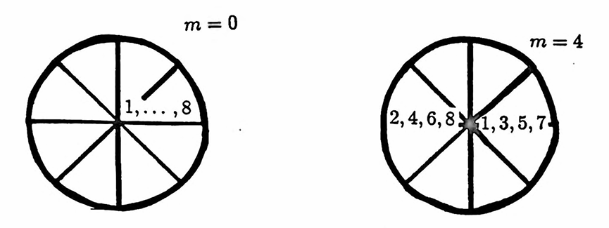
When $\,m = 0\,,$ no ‘genuine’ complex products are involved:

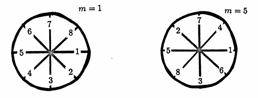
$$ \text{DFT}(0) = y_1 + \cdots + y_N $$

When $\,m = 1\,,$ the exponents $\,-2\pi(1)(n-1)/8\,$ in the exponential cause movement backward around the unit circle, one step at a time, as $\,n\,$ goes from $\,1\,$ to $\,N\,.$ For example, $\,y_4\,$ must multiply the exponential at an angle of $\,-2\pi(1)(4-1)/8 = -3\pi/4\,.$

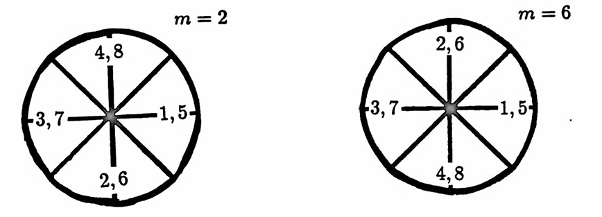
When $\,m = 2\,,$ one moves backward around the unit circle, two steps at a time , so that, e.g., now $\,y_4\,$ must multiply the exponential at an angle of $\,-2\pi(2)(4-1)/8 = -3\pi/2\,.$

How much redundancy?

Now, the number of distinct complex products that must be computed can be counted. The products at angles $\,0\,$ and $\,\pi\,$ are not truly complex, since $\,e^{0i} = 1\,$ and $\,e^{\pi i} = -1\,$; so these will not be counted as complex products.

At $\,\theta = 2\pi(1)/8\,,$ there are $\,4\,$ distinct complex products $\,(n = 2, 4, 6, 8)\,.$
At $\,\theta = 2\pi(2)/8\,,$ there are $\,6\,$ $\,(n = 2, 3, 4, 6, 7, 8)\,.$
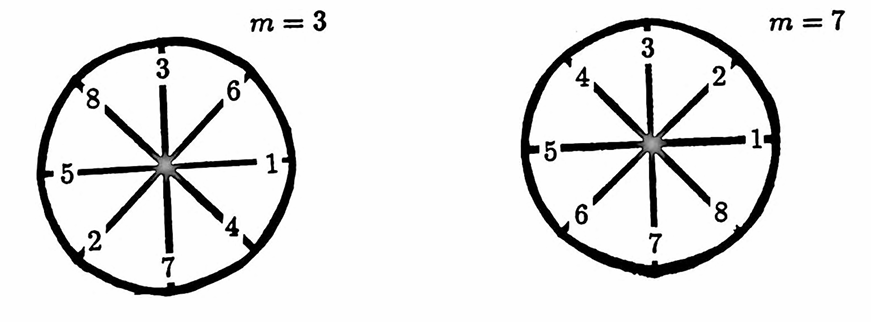
At $\,\theta = 2\pi(3)/8\,,$ there are $\,4\,$ $\,(n = 2, 4, 6, 8)\,.$
At $\,\theta = 2\pi(5)/8\,,$ there are $\,4\,$ $\,(n = 2, 4, 6, 8)\,.$
At $\,\theta = 2\pi(6)/8\,,$ there are $\,6\,$ $\,(n = 2, 3, 4, 6, 7, 8)\,.$
At $\,\theta = 2\pi(7)/8\,,$ there are $\,4\,$ $\,(n = 2, 4, 6, 8)\,.$

Thus, computation of the entire DFT actually requires only $\,4 + 6 + 4 + 4 + 6 + 4 = 28\,$ distinct complex products.

The MATLAB command fft is an efficient computation of the DFT, that (at least partially) eliminates the redundancy illustrated here.

Uniform Hypotheses for the following Propositions

The next few propositions develop the relationship between the DFT and the periodogram (Section $2.6$). In these propositions, the following situation is assumed to hold:

$N\,$ is a positive integer.
$\{(t_i,y_i)\}_{i=1}^N\,$ is a data set with a time list $\,(t_1,\ldots,t_N)\,$ that is uniform with positive increment $\,\Delta T\,.$ All values of $\,t_i\,$ and $\,y_i\,$ are real numbers.
$K\,$ is the largest integer satisfying $\,N \ge 2K + 1\,.$
If $\,N\,$ is odd, then $\,N = 2K + 1\,,$ so that $\,K =\frac{N-1}2\,.$
If $\,N\,$ is even, then $\,N = 2K + 2\,,$ so that $\,K =\frac{N-2}2\,.$
The numbers $\,a_0,a_1,b_1,\ldots,a_K,b_K\,$ are the coefficients of the discrete Fourier series corresponding to the data set .
The numbers $\,\text{DFT}(m)\,,$ for $\,m = 0,\ldots,, N-1\,,$ are the $\,N\,$ independent values of the discrete Fourier transform.

Proposition

$$\text{DFT}(0) = N\cdot a_0\,,$$

and

$$ \begin{gather} \text{DFT}(m) = e^{i\frac{2\pi mt_1}P}\cdot \frac N2(a_m - ib_m)\,,\cr \text{for}\ \ m = 1,\ldots,K \end{gather} $$

Proof

First, define a function $\,g\,$ via:

$$ g(t_n,m) := \sum_{n=1}^N y_n e^{-i\frac{2\pi mt_n}P} $$

Observe that:

$$ \begin{align} &g(t_n - t_1,m)\cr\cr &\quad = \sum_{n=1}^N y_n e^{-i\frac{2\pi m(t_n-t_1)}P}\cr\cr &\quad = \sum_{n=1}^N y_n e^{-i\frac{2\pi m(n-1)\Delta T}{N\Delta T}}\cr\cr &\quad = \text{DFT}(m) \end{align} $$

and

$$ \begin{align} &g(t_n - t_1,m)\cr\cr &\quad = \sum_{n=1}^N y_n e^{-i\frac{2\pi m(t_n-t_1)}P}\cr\cr &\quad = e^{i\frac{2\pi mt_1}P}\sum_{n=1}^N y_n e^{-i\frac{2\pi m t_n}P}\cr\cr &\quad = e^{i\frac{2\pi mt_1}P}\,\cdot\, g(t_n,m) \end{align} $$

Combining these results yields:

$$ \text{DFT}(m) = e^{i\frac{2\pi mt_1}P}\,\cdot\, g(t_n,m) $$

Now:

$$ \begin{align} &g(t_n,m)\cr\cr &\quad := \sum_{n=1}^N y_n e^{-i\frac{2\pi mt_n}P}\cr\cr &\quad = \sum_{n=1}^N y_n \left[ \cos\bigl(\frac{2\pi mt_n}P\bigr) - i\sin\bigl(\frac{2\pi mt_n}P\bigr) \right]\cr\cr &\quad = \sum_{i=1}^N y_n\cos\bigl( \frac{2\pi mt_n}P \bigr) - i\sum_{n=1}^N y_n\sin\bigl(\frac{2\pi mt_n}P\bigr)\cr\cr &\quad = \frac N2 \left[ \frac 2N \sum_{n=1}^N y_n\cos\bigl(\frac{2\pi mt_n}P\bigr) \right]\cr\cr &\qquad - i\frac N2\left[ \frac 2N\sum_{n=1}^N y_n\sin\bigl( \frac{2\pi mt_n}P\bigr) \right] \end{align} $$

When $\,m = 0\,$:

$$ \begin{align} \text{DFT}(0) &= e^{i\frac{2\pi(0)t_1}P}\,\cdot\,g(t_n,0)\cr\cr &= N\left[ \frac 1N\sum_{n=1}^N y_n \right]\cr\cr &= N\cdot a_0 \end{align} $$

For $\,m = 1,\ldots,K\,$:

$$ \begin{align} \text{DFT}(m) &= e^{i\frac{2\pi mt_1}P}\,\cdot\,g(t_n,m)\cr\cr &= e^{i\frac{2\pi mt_1}P}\,\cdot\,\frac N2(a_m - ib_m)\ \ \ \blacksquare \end{align} $$

The previous proposition describes the first half of the DFT list

With this proposition, the first half (approximately) of the $\,N\,$ DFT values has been described in terms of the discrete Fourier series coefficients. The next proposition shows that the remaining DFT values are completely described in terms of the first half. The following sketches illustrate the situation when $\,N\,$ is even, and when $\,N\,$ is odd.

Proposition

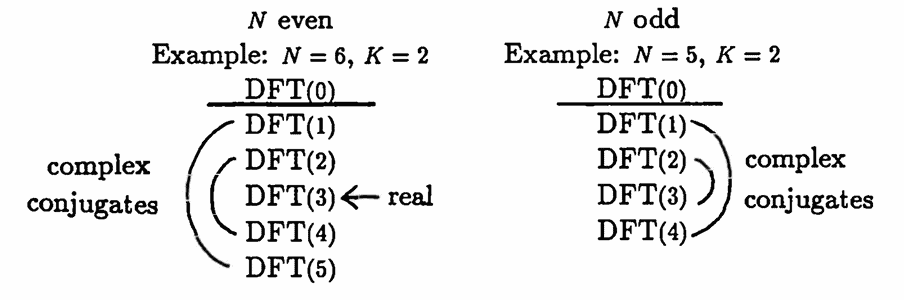
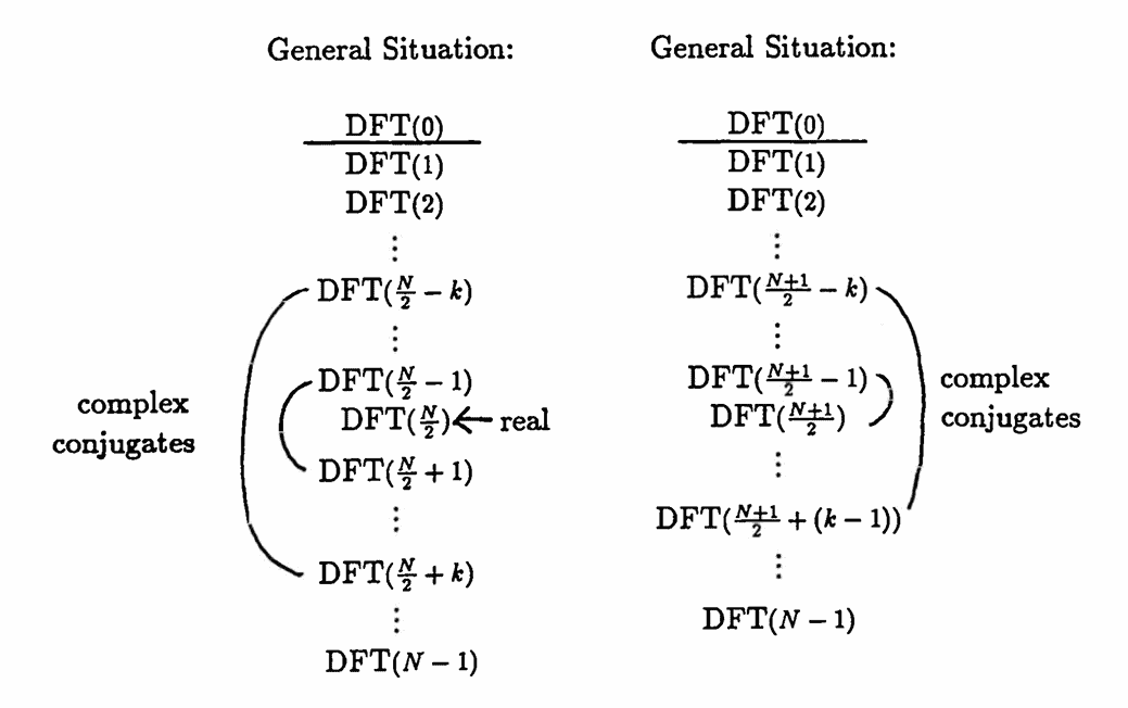
When $\,N\,$ is even, then $\,\text{DFT}(\frac N2 - k)\,$ and $\,\text{DFT}(\frac N2 + k)\,$ are complex conjugates, for $\,k = 1,\ldots,K\,.$ Also, $\,\text{DFT}(\frac N2)\,$ is a real number:

$$ \text{DFT}(\frac N2) = y_1 - y_2 + y_3 - y_4 + \cdots + y_{N-1} - y_N $$

When $\,N\,$ is odd, then $\,\text{DFT}\bigl(\frac{N+1}2 - k\bigr)\,$ and $\,\text{DFT}\bigl(\frac{N+1}2 + (k-1)\bigr)\,$ are complex conjugates, for $\,k = 1,\ldots,K\,.$

Proof

$N\,$ even

Suppose first that $\,N\,$ is even. Let $\,m = \frac N2 \pm k\,,$ and let $\,\text{Re}(z)\,$ denote the real part of a complex number $\,z\,.$ Then:

$$ \begin{align} \text{Re}\bigl( &e^{-i\frac{2\pi(\frac N2\pm k)(n-1)}N}\bigr)\cr\cr &\quad = \text{Re} \bigl( e^{-i\bigl(\pi(n-1)\pm\frac{2\pi k(n-1)}N\bigr)}\bigr)\cr &\quad = \cos\bigl( \pi(n-1) \pm \frac{\overbrace{2\pi k(n-1)}^{:= K}}N \big)\cr\cr &\quad = \cos( \pi(n-1))\cos K \mp \sin(\pi(n-1))\sin K\cr\cr &\quad = \cos(\pi(n-1))\cos K \end{align} $$

It follows that the real parts of $\,\text{DFT}\bigl(\frac N2 + k\bigr)\,$ and $\,\text{DFT}\bigl(\frac N2 - k\bigr)\,$ are the same.

Continuing, let $\,\text{Im}(z)\,$ denote the imaginary part of a complex number $\,z\,.$ Then:

$$ \begin{align} \text{Im}\bigl( &e^{-i\frac{2\pi(\frac N2\pm k)(n-1)}N}\bigr)\cr\cr &\quad = \text{Im} \bigl( e^{-i\bigl(\pi(n-1)\pm\frac{2\pi k(n-1)}N\bigr)}\bigr)\cr &\quad = -\sin\bigl( \pi(n-1) \pm \frac{\overbrace{2\pi k(n-1)}^{:= K}}N \big)\cr\cr &\quad = -[\sin( \pi(n-1))\cos K \pm \cos(\pi(n-1))\sin K]\cr\cr &\quad = \mp\cos(\pi(n-1))\sin K \end{align} $$

In particular, the imaginary parts of $\,\text{DFT}\bigl(\frac N2 + k\bigr)\,$ and $\,\text{DFT}\bigl(\frac N2 - k\bigr)\,$ have opposite signs. This shows that $\,\text{DFT}\bigl(\frac N2 - k\bigr)\,$ and $\,\text{DFT}\bigl(\frac N2 + k\bigr)\,$ are complex conjugates, when $\,N\,$ is even.

When $\,m = \frac N2\,,$ one has

$$ \begin{align} &\text{DFT}\bigl(\frac N2\bigr)\cr\cr &\quad = \sum_{n=1}^N y_n e^{-i\frac{2\pi\frac N2(n-1)}N}\cr\cr &\quad = \sum_{n=1}^N y_n e^{-i\pi(n-1)}\cr\cr &\quad = y_1 - y_2 + y_3 - y_4 + \cdots + y_{N-1} - y_N\,, \end{align} $$

since $\,e^{-i\pi(n-1)}\,$ is alternately $\,+1\,$ and $\,-1\,.$

$N\,$ odd

Next, let $\,N\,$ be odd. Write:

$$ \begin{gather} \frac{N+1}2 - k = \frac N2 - (k - \frac 12)\cr\cr \text{and}\cr\cr \frac{N+1}2 + (k-1) = \frac N2 + (k - \frac 12) \end{gather} $$

Replacing $\,k\,$ by $\,k - \frac 12\,$ in the previous arguments completes the proof. $\blacksquare$

The next result relates the discrete Fourier transform to the periodogram.

Proposition

Let $\,\bar z\,$ denote the complex conjugate of a complex number $\,z\,.$ Then: $$ \begin{gather} \sqrt{ \text{DFT}(m) \cdot \overline{\text{DFT}(m)} } = \frac N2\sqrt{a_m^2 + b_m^2}\ \,,\cr\cr m = 1,\ldots,K \end{gather} $$

Proof

Ket $\,K := \frac{2\pi mt_1}P\,,$ and recall that for complex numbers $\,z_1\,$ and $\,z_2\,,$ $\,\overline{z_1z_2} = \overline{z_1}\cdot \overline{z_2}\,.$ Then:

$$ \begin{align} &\sqrt{\text{DFT}(m)\cdot \overline{\text{DFT}(m)}}\cr\cr &\quad = \sqrt{ e^{i\frac{2\pi mt_1}P}\frac N2(a_m - ib_m) \cdot \overline{e^{i\frac{2\pi mt_1}P}\frac N2(a_m - ib_m)} }\cr\cr &\quad = \sqrt{ e^{iK}\frac N2(a_m-ib_m)e^{-iK}\frac N2(a_m + ib_m)}\cr\cr &\quad = \frac N2\sqrt{a_m^2 + b_m^2}\ \ \ \ \blacksquare \end{align} $$

The periodogram in terms of the DFT

Consequently, the periodogram can be written as:

$$ \left\{ \left( \frac Pk\,,\, \sqrt{\text{DFT}(k)\cdot\overline{\text{DFT}(k)}}\right)\ |\ k = 1,\ldots,K \right\} $$

Time savings: 2 min 50 sec versus 6 sec

Since the built-in MATLAB commands for implementing the DFT are so efficient, computation of the periodogram via the DFT provides a great time-savings.

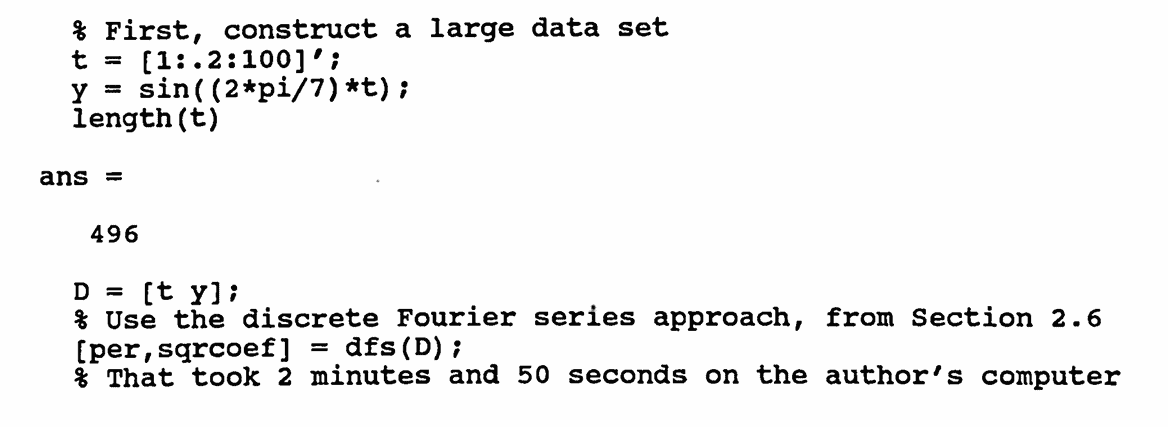
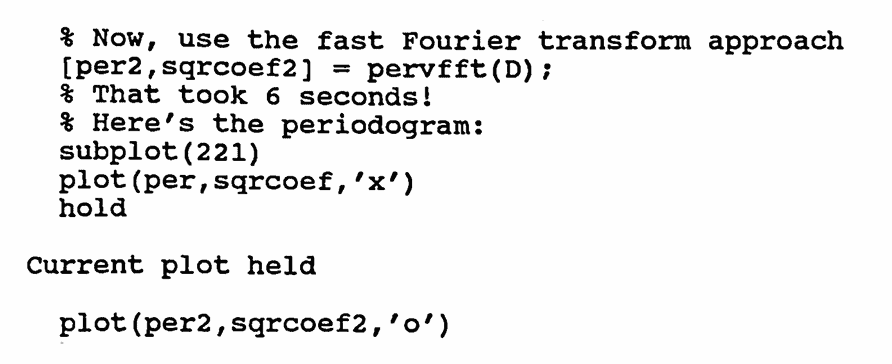
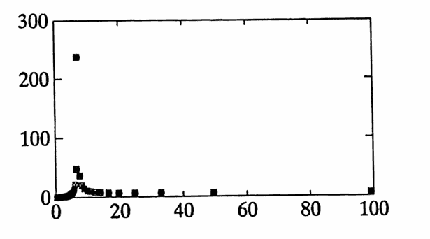
The MATLAB example at the conclusion of this section first computes the periodogram corresponding to a large data set ($\,496\,$ points) using the discrete Fourier series approach, from Section $2.6\,.$ This took $\,2\,$ minutes and $\,50\,$ seconds on the author's computer. However, finding the same periodogram by using MATLAB's built-in commands for the DFT, and exploiting the relationship between the DFT and the periodogram, took only $\,6\,$ seconds!

MATLAB Implementation: Finding the Periodogram, Using a Fast Fourier Transform

MATLAB FUNCTION
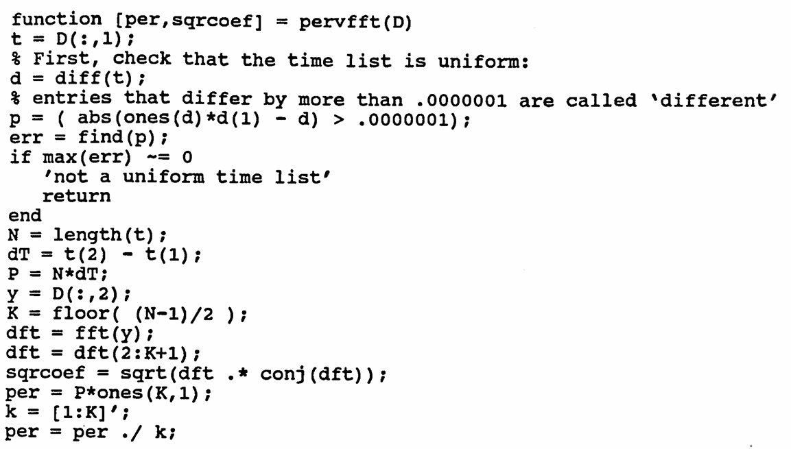
pervfft(D)

The following MATLAB function finds the periodogram corresponding to a data set (with the maximum allowable value of $\,K\,$), by using the built-in MATLAB fft command to find the DFT, and then computing the values:

$$ \left\{ \left( \frac Pk\,,\, \sqrt{\text{DFT}(k)\cdot \overline{\text{DFT}(k)}} \right)\ |\ k = 1,\ldots,K \right\} $$

To use the function, type:
[per,sqrcoef] = pervfft(D);

The name ‘pervfft’ stands for ‘ periodogram via a fast Fourier transform ’.

Required input, D

The required input is a data set $\,\{(t_i,y_i)\}_{i=1}^N\,,$ with $\,N \ge 3\,.$ The time values must be stored in a column vector t and the corresponding data values in a column vector y . Then, D = [t,y] is the $\,N \times 2\,$ matrix containing the data set.

The time list contained in t must be uniform (increment $\,\Delta T \gt 0\,$). The program begins by checking that this requirement is met; if not, the program is halted and the message ‘not a uniform time list’ is displayed. (As written, increments between time values are said to ‘differ’ if they differ by more than $\,0.0000001\,.$ This value may be changed for different tolerances.)

Outputs:
per
sqrcoef

The output per is a column vector containing the periods $\,P,\frac P2,\frac P3,\ldots,\frac Pk\,,$ where $\,P = N\Delta T\,.$

The output sqrcoef is a column vector containing the numbers

$$ \sqrt{ \text{DFT}(k)\cdot \overline{\text{DFT}(k)} } = \frac N2\sqrt{a_k^2 + b_k^2}\,, $$

for $\,k = 1,\ldots,K\,.$

The periodogram is then obtained with the command:
plot(per,sqrcoef)

OCTAVE requires two changes:

You must write
ones(size(d))
instead of
ones(d)
The last line of the function must be:
endfunction

MATLAB Example

The following example gives a time-comparison between computing the periodogram via the program in Section $2.6$, and via a fast Fourier transform.

Matlab Example: time comparison; periodogram

The line ‘subplot(221)’ is optional; omit it if you don't need a grid of smaller plots. Recall that

subplot(22x)

enables a $\,2\times 2\,$ grid of plots, with the position in this grid determined by the value of x :

Value of x	Position in grid
$1$	first row, first column
$2$	first row, second column
$3$	second row, first column
$4$	second row, second column

When I put my dissertation online in the year $2025$, both functions (dfs and pervfft) ran this example in less time than it took me to blink—a testament to increased computing speeds over the decades!